Numerical solution of ordinary differential equations
In ordinary differential equations the unknown function depends only on one variable. Therefore only ordinary derivatives of the function in this one variable can occur. The order of the differential equation is the highest occurring derivative. One differentiates between explicit and implicit differential equations, depending on whether you can solve the equation for the highest occurring derivative or not.
In application, often the time is the variable. Thus, the differential equation describing the changing behavior of the required quantities.
Only for a few differential equations exist explicit algorithms to solve. For many solutions is not even an explicit solution representation possible so that here much resorting to numerical approximation.
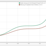
This is the simplest form of an explicit one-step method. In each step, the change specified by the differential equation is determined, and this is used to determine the next step. In practical terms, the change rule is integrated in each step using the left-hand side rectangle rule. The explicit Euler method can also be regarded as a first-order Runge-Kutta method.
The Heun method is a simple method belonging to the class of Runge-Kutta methods. In each step, the differential equation is evaluated multiple times: at the current point and at the next point specified by the explicit Euler method. Both results are averaged and used in the next step. In practical terms, the rate of change is integrated in each step using the trapezoidal rule. This is a two-stage explicit Runge-Kutta method of order 2.
Another second-order Runge-Kutta method. The differential equation is now evaluated multiple times at each step, namely at the current point and at the next point specified by the explicit Euler method. However, only the last evaluation is carried over to the next step (unlike in Heun’s method). This is a two-stage explicit Runge-Kutta method of second order.
The differential equation is now evaluated multiple times at each step: at the current point, at an intermediate point, and at the next point. All three values are weighted and incorporated into the next step. In practical terms, the change rule is integrated at each step using Simpson’s rule. This is a 3-step explicit Runge-Kutta method of order 3.
The differential equation is now evaluated multiple times at each step: once at the current point, twice at an intermediate point, and once at the next point. All four values are weighted and incorporated into the next step. This is a 4-step explicit Runge-Kutta method of order 4.