

Probability distributions
Most pratical relevant probability distributions can be divided in the two area discrete and continuous. Discrete probability distributions describe random experiments in which the result set is at most countable (for example the eyes count when rolling a dice). They assign individual, concrete outputs of the experiment to positive probabilities. Continuous probability distributions describe random experiments in which the result set is continuous, e.g. represents a times. In this case the probability for each time is 0 and only statements can be made about how likely it is that the result is in a specified interval.
Discrete probability distributions
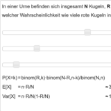
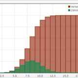
With the help of discrete probability distributions one can model the probabilities that result in urn models.
In an urn there are well mixed N balls. Among the balls are R red and N-R white balls. n balls are randomly drawn of the urn. This raises the question: What is the probability that there are exactly k (k≤n, k≤R) red ball among n balls drawn? In answering this question, the two cases that each ball drawn is immediately put back into the urn and that once drawn balls are put aside have to be distinguished (sampling with and without replacement).
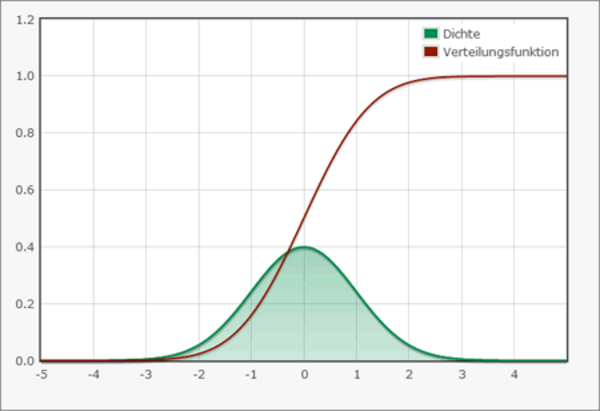
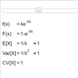
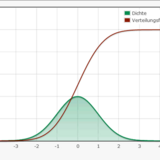
Continuous probability distributions
With the help of continuous probability distributions problems can be modeled, where the random variable can take any value in an interval (for example, the waiting time of customers, the life time of a component, etc.). Since each concrete value (e.g., a specific time) will be assigned the probability of 0, no discrete probability distributions can be used for such problems, but continuous probability distributions with densities hase to be used.
Interactive pages about probability distributions
Extended version
An extended version of the info page above is available as probability distributions webapp.